1 Introduction
- After first outlining some of the useful applications of trajectory similarity measures, four of the most commonly used similarity measures will be discussed in detail: longest common subsequence (LCSS), Fréchet distance, dynamic time warping (DTW), and edit distance
- These four measures have been implemented within a new R package called “SimilarityMeasures,” available on CRAN
2 Applications of trajectory similarity measures
- 1) Database indexing
- The most common use of trajectory similarity measures
- Vlachos et al. - the longest common subsequence similarity measure - indexed marine animal trajectories
- 2) Vehicle and pedestrian traffic
- Buchin et al. - Fréchet and discrete Fréchet similarity measures - detected commuting pattern
- Li et al. - longest common subsequence similarity measure - compared calculated paths with actual paths
- 3) Sports
- Haase and Brefeld - dynamic time warping similarity measure - explored similar movements in a soccer game
- Perše et al. - edit distance similarity measure - analyzed and segmented basketball games
3 Trajectory similarity computation
- A trajectory TA, contains a series of m timestamped n dimensional points ai=(ai,1,...,ai,n):
TA=((t1,a1),...,(tm,am))
- The length of a trajectory is defined as the number of discrete timestamps ("fixes")
- The key challenge in identifying a satisfactory trajectory similarity measure is the arbitrary nature of the discretization
3.1 Fréchet metric
[Attributes]
- The most popular similarity measures
- Can be applied to both continuous directed curves as well as the discretized trajectories
- The Fréchet metric is the minimum leash length required to complete the traversal of both human and dog curves

[Pros]
- Trajectory points are not matched together allowing the metric to perform well with even the most widely varying sampling rates and trajectory lengths
[Cons]
- Can be greatly affected by outliers because every point of the two trajectories is used in the calculation
3.2 Dynamic time warping (DTW)
[Attributes]
- Relies on matching points in trajectories
- The trajectories are "warped" in a non-linear way to measure similarity allowing for varying sampling rates
- A common warping cost is the total of all distances calculated along the warping path and the similarity value is the minimum of all possible warping costs
[Pros]
- A single point on one trajectory can be matched to multiple points on the other allowing to perform well with trajectories of different lengths and even widely varying sampling rates
[Cons]
- Outliers can again greatly affect this method because every point of both trajectories must have at least one match
DTW란?
DTW는 두 개의 궤적(혹은 경로)이 얼마나 유사한지를 측정하는 방법입니다. 궤적이란 시간에 따라 변하는 두 점의 움직임을 말해요. 예를 들어, 한 사람이 걸어가는 경로와 다른 사람이 뛰어가는 경로를 비교할 때 사용될 수 있습니다.
DTW가 왜 유용한가? 두 사람이 같은 길을 걷고 있어도, 한 사람은 빠르게 걷고 다른 사람은 느리게 걸을 수 있죠. DTW는 이처럼 시간의 차이를 고려하여 궤적을 비교할 수 있습니다. 그래서 궤적의 길이나 속도가 달라도 비슷한 패턴을 찾을 수 있습니다.
어떻게 계산되나?
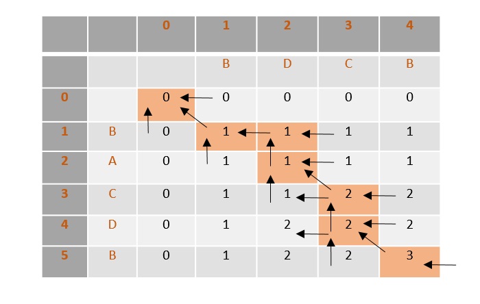
- 거리 행렬 생성:
두 궤적이 있다고 할게요. 궤적 A의 길이가 5, 궤적 B의 길이가 4라면, 5x4 크기의 격자를 만듭니다. 이 격자의 각 점은 A의 특정 위치와 B의 특정 위치 사이의 거리를 나타냅니다. 일반적으로 유클리드 거리를 사용해 각 지점 간의 거리를 계산해요. - 워핑 경로(Warping Path):
궤적 A와 B 사이의 거리를 따져가며, 격자 위에서 가장 최적의 경로를 찾습니다. 이 경로는 시작점 (1,1)에서 끝점 (m,k)까지 갑니다. 예를 들어 (1,1)에서 출발했다면, 한 번에 한 칸씩만 이동하면서 (1,2), (2,1), (2,2) 중 한 곳으로 이동할 수 있습니다. - 워핑 비용(Warping Cost):
경로마다 비용을 계산합니다. 비용은 경로를 따라 이동하며 계산한 거리들의 합입니다. 이때 모든 가능한 경로들 중에서 가장 적은 비용을 찾는 것이 목적입니다.
DTW가 좋은 이유
- 길이가 다른 궤적도 비교 가능: DTW는 궤적의 길이가 달라도 비교할 수 있습니다. 예를 들어, 궤적 A가 100개 지점으로 이루어져 있고, 궤적 B가 50개 지점으로 이루어져 있어도 괜찮습니다.
- 속도가 달라도 유사한 패턴 찾기 가능: 한 궤적에서 한 점이 여러 점과 비교될 수 있기 때문에, 속도가 달라도 비슷한 움직임을 찾아낼 수 있습니다.
DTW의 단점
- 이상치(outliers) 문제: 궤적의 모든 점들이 반드시 짝을 이루어야 하므로, 일부 이상치(잘못된 데이터나 극단적인 움직임)가 전체 결과에 큰 영향을 줄 수 있습니다.
- 거리 계산 방식의 중요성: 두 점 사이의 거리를 계산하는 방법에 따라 결과가 크게 달라질 수 있습니다.
요약
DTW는 시간의 차이가 있더라도 두 궤적을 비교할 수 있는 방법입니다. 주어진 두 궤적의 모든 점을 비교해 가장 적은 비용의 경로를 찾고, 그 경로의 거리 합이 유사도를 나타냅니다.
3.3 Longest common subsequence (LCSS)
[Attributes]
- Trajectories can be stretched, while some points can remain unmatched
- The LCSS value represents a count of the maximum number of points that can be considered equivalent, while the trajectories are traversed monotonically from start to end
[Formular]
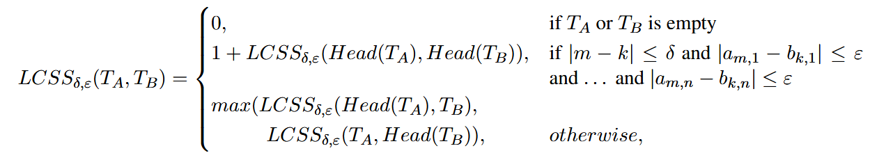
- The constant δ provides a maximum index difference when comparing points from the two trajectories.
- The constant ε defines the maximum distance in each dimension allowed for two points to be considered equivalent
- Head(TA) represents TA with the last point removed
[Pros]
- With careful use of the two constants, δ and ε, this method is highly robust to outliers, while performing well with trajectories of different lengths
- Generally functions well with different sampling rates
[Cons]
- Widely varying sampling rates may cause issues when many points must be left unmatched in the calculation
[알고리즘] 그림으로 알아보는 LCS 알고리즘 - Longest Common Substring와 Longest Common Subsequence
LCS는 주로 최장 공통 부분수열(Longest Common Subsequence)을 말합니다만, 최장 공통 문자열(Longest Common Substring)을 말하기도 합니다.
velog.io
Longest Common Subsequence (LCSS)는 두 궤적(trajectory)의 유사성을 측정하는 방법입니다. LCSS는 궤적 간의 비슷한 부분을 찾아내는데, 일부 점들이 짝을 이루지 않아도 된다는 특징이 있습니다. 이를 통해 궤적의 길이가 다르거나 일부 데이터가 부족해도 유사성을 정확하게 분석할 수 있습니다.
최장 공통 부분수열(LCSS)의 기본 개념
LCSS는 두 궤적에서 가장 많이 겹치는 점들의 개수를 계산하는 방법입니다. 예를 들어, 궤적 A와 궤적 B가 있으면, 이 궤적들이 시작부터 끝까지 순차적으로 비교됩니다. 두 궤적에서 "동일"하다고 간주할 수 있는 점이 몇 개 있는지를 계산하여 유사도를 측정합니다.
핵심 개념:
- 궤적의 일부분 무시 가능: 궤적 A나 B에서 몇몇 점들은 짝이 이루어지지 않아도 괜찮습니다. 이를 통해 유사성이 없는 부분이나 이상치(outliers)를 무시할 수 있습니다.
- 단순 거리 계산이 아님: DTW처럼 모든 점을 비교하는 것이 아니라, 두 궤적에서 가장 많이 일치하는 점들을 찾아내는 것이 핵심입니다.
- 정확한 비교를 위한 두 가지 기준:
- δ (델타): 두 궤적을 비교할 때, 어느 정도 차이가 있어도 괜찮다는 범위를 설정합니다. 예를 들어, 궤적 A의 1번 지점과 궤적 B의 3번 지점이 비교될 수 있는 범위.
- ε (엡실론): 두 궤적의 점들이 얼마나 가까워야 "일치"한다고 볼지를 결정하는 기준입니다. 즉, 두 점 사이의 거리가 이 값보다 작아야 동일한 점으로 간주됩니다.
예시
궤적 A와 궤적 B가 있을 때, 특정 점들이 ε 값 이하로 가까우면 같은 점으로 간주하고, δ 값만큼의 차이가 있어도 같은 시간대로 인정됩니다. 두 궤적에서 일치하는 점들이 많으면 많을수록, LCSS 값이 커집니다.
장점
- 이상치에 강함: LCSS는 일부 점들을 무시할 수 있어서, 잘못된 데이터나 극단적인 움직임이 있는 경우에도 정확한 유사성을 측정할 수 있습니다.
- 다른 길이의 궤적 비교 가능: 궤적의 길이가 달라도 비교할 수 있고, 다른 속도로 기록된 데이터를 비교할 때도 유리합니다.
단점
- 샘플링 비율 문제: 궤적의 샘플링 속도가 너무 다를 경우, 많은 점들이 비교되지 않을 수 있습니다.
요약
LCSS는 두 궤적에서 가장 많이 일치하는 점들을 찾아 그 개수로 유사성을 측정하는 방법입니다. 델타(δ)와 엡실론(ε)이라는 두 가지 기준을 사용해 얼마나 큰 차이를 허용할지를 설정할 수 있어서, 길이가 다르거나 일부 이상치가 있는 궤적도 잘 비교할 수 있습니다.
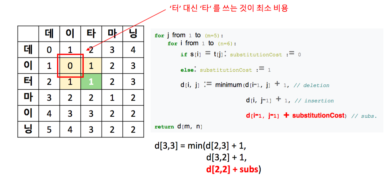
3.4 Edit distance
[Attributes]
- Count the minimum number of edits required to make two trajectories equivalent
[Pros]
- Relatively be unaffected by outliers because the matching threshold reduces the increments to values of 0 and 1 only
- Also performs well with trajectories that have varying sampling rates
[Cons]
- Different length trajectories will automatically inflate the edit distance because every extra point is required to be edited out (or in) for the trajectories to be considered equivalent
4 Comparison and evaluation
4.1 Normalization
- Each pair of trajectories was normalized to approximately match by rotating, scaling, and translating to align their start and end points
4.2 The similarity measures
- There is a strong (positive) correlation between Fréchet distance and DTW ratio similarity values, while a strong (negative) correlation can be seen between LCSS ratio and edit distance ratio
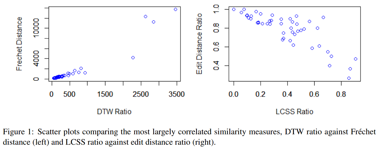
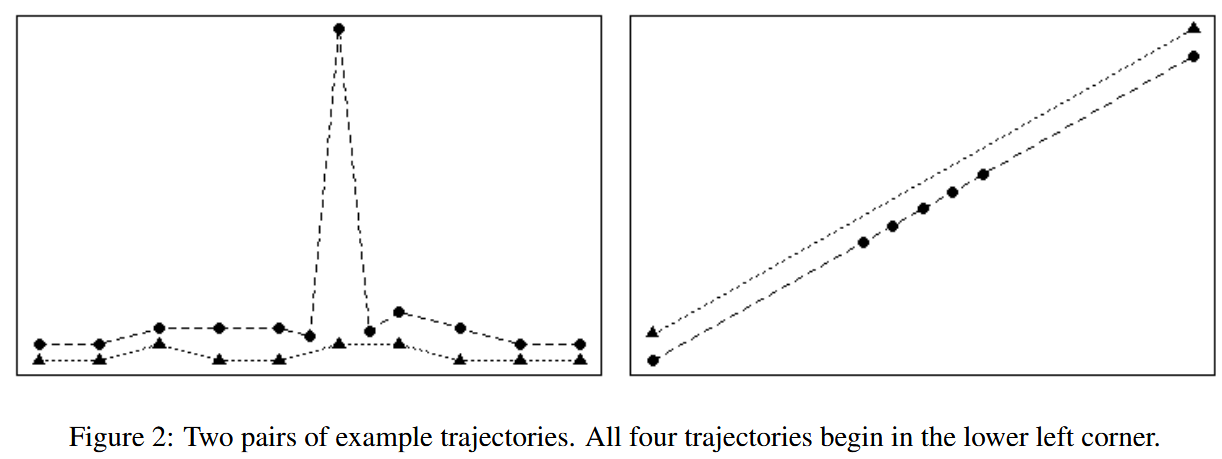
- A peak in the left image will not influence the DTW value greatly, but the Fréchet distance will reflect considerable dissimilarity in this pair of trajectories
- In the right image, LCSS will consider these trajectories perfectly equivalent because all of one trajectory points are matched up. However, edit distance highlights that the five middle points have no match and therefore the trajectories are quite dissimilar